Assay development guidelines

This topic provides guidelines for adjusting the protocol, and notes about the utility.
Note: See the Labware Reference Guide for labware-specific maximum well capacity and other details. You can find this guide in the Literature Library page of the Protein Sample Prep Workbench.
Correcting for loss due to evaporation
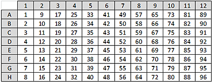
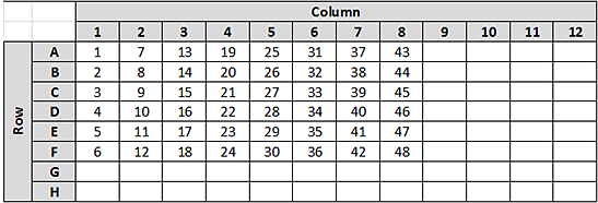
Evaporation can cause problems for any normalization process, whether conducted manually or using automation. The time difference between the normalization of the first sample (A1) and the last sample (H12), leads to progressively increasing atmospheric exposure across the samples. This causes a gradual increase in the mass of sample that is transferred into the normalized sample plate, which leads to higher than expected concentrations for samples with long exposure times. The following figure shows the order in which the Normalization utility normalizes the samples. The utility starts with column 1 on the left and finishes with column 12 on the right. Without any evaporation correction, you would expect to see the normalized concentrations increase across the plate from left to right.
Figure Run order: the sequence in which samples are normalized
 |
Step 11 of the Normalization Method Setup Tool contains an optional Evaporation Correction Factor to correct for this problem. The tool applies the factor to the calculated normalization volumes. The factor progressively decreases the volume of Initial Sample (deck location 2) that is used to prepare each normalized sample (deck location 6). This reduction in sample volume is then substituted with diluent to maintain the same target volume.
The Evaporation Correction Factor represents the relative increase in concentration across an entire plate of 96 samples. For example, if the target concentration is 1.00 mg/mL, and after normalization A1 = 1.00 mg/mL and H12 = 1.05 mg/mL, then the relative increase in concentration across the plate would be 0.05 or 5%. Thus, the recommended Evaporation Correction Factor would be 5%.
How to determine an appropriate Evaporation Correction Factor
To determine an appropriate percentage to use for the Evaporation Correction Factor, run a representative normalization protocol to determine the amount of concentration increase observed. The representative normalization run can use an inexpensive reagent, such as bovine serum albumin (BSA). Example 1 describes how to determine the Evaporation Correction Factor from a full plate of normalized results.
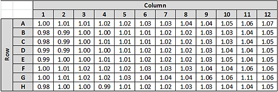
Example 1. Determining the Evaporation Correction Factor from a full plate of normalization results.
• Target Concentration = 1.0 mg/mL
• Normalization Run Results:
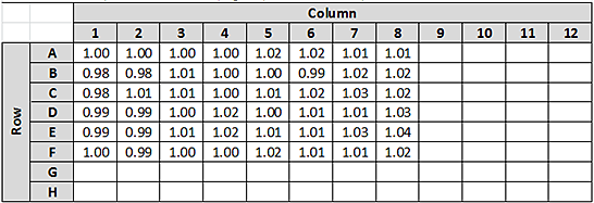
Figure Example 1 normalized sample concentration (mg/mL) without an Evaporation Correction Factor
 |
To calculate the Evaporation Correction Factor for Example 1:
1 Use the following equation to calculate relative inaccuracy (RI) for each of the 96 samples with respect to the target concentration:
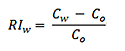 |
where,
RIw is the relative inaccuracy for well location w
Cw is the concentration for well location w
Co is the target concentration
2 Plot the relative inaccuracy (RI) values against sample number (n), along with a linear regression line.
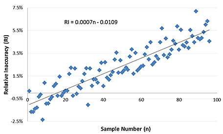 |
3 The equation for the regression line is used to solve for RI when n = 96. This gives the relative increase in concentration across the plate, and thus the recommended Evaporation Correction Factor. The calculated factor for this example is as follows:
Evaporation Correction Factor = 0.0007 × 96-0.0109 = 0.056 = 5.6%
The same process can be followed when using a partial plate of normalized samples, as Example 2 demonstrates.
Example 2: Determining the Evaporation Correction Factor from a partial plate of normalization results.
• Target Concentration = 1.0 mg/mL
• Normalization Run Results for Partial Plate:
Figure Example 2 normalized sample concentration (mg/mL) without an Evaporation Correction Factor
 |
To calculate the Evaporation Correction Factor for Example 2:
1 Calculate the relative inaccuracy (RI) for each of the 48 samples with respect to the target concentration. See Example 1 for the equation to calculate RI.
2 Plot the relative inaccuracy (RI) values against sample number (n), along with a linear regression line. The following figures show how the sample number (n) would change for this partial plate example.
Figure
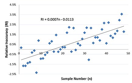 |
Figure Sample run order: sequence in which the samples were normalized
 |
3 The equation for the regression line is used to solve for RI when n = 96. This gives the relative increase in concentration across the plate, and thus the recommended Evaporation Correction Factor.
Evaporation Correction Factor = 0.0007 × 96-0.0113 = 0.056 = 5.6%
Note: Even though only 48 sample were run in this example, the Evaporation Correction Factor is still calculated by solving the regression equation for n = 96. This is because the Evaporation Correction Factor is expressed as the percent increase across an entire plate of 96 samples. Because we don't have a full plate of results, the correction factor must be determined by extrapolation.
Conditions that can affect evaporation
Three factors that are known to affect the evaporation that is observed when using the Normalization utility are:
1 Atmospheric conditions in the laboratory
The temperature and humidity of a laboratory affect the amount of evaporation that is observed with samples that are exposed to atmosphere. Many laboratories have environmental management systems to help maintain constant atmospheric conditions. These environmental controls will help to reduce changes in the amount of evaporation that is observed, but slight changes in the Evaporation Correction Factor may be required to maintain a consistent normalization results, especially with changing seasons.
2 Sample Plate labware type
The Initial Sample Plate labware type can have a significant impact on the amount of evaporation that is observed. Different well geometries and volume capacities can impact the rate of evaporation that will be observed.
• Well geometry. Plates with larger diameter wells provide greater surface area for interaction with the open atmosphere, leading to faster evaporation rates.
• Volume capacity. Consider a scenario where Plate 1 has a 100-µL capacity and Plate 2 has a 10-µL capacity. If both plates lose 5 µL of diluent to evaporation, the resulting concentration in Plate 1 would increase by a factor of ~1.05, while the concentration in Plate 2 would increase by a factor of 2.
3 Solvent
The solvent in which the sample is suspended will dramatically affect the evaporation rate. When determining the evaporation rate, use the same sample solvent that will be used during the normalization run using real samples.
Pipetting accuracy and liquid classes
The following table lists the default liquid classes that the Normalization utility uses.
Liquid class name | When to use this liquid class |
|---|---|
AM_Normalization_diluent_20-150ul | High-volume transfers of diluent (20 to 150 µL) |
AM_Normalization_diluent_5-20ul | Low-volume transfers of diluent (5 to 20 µL) |
AM_Normalization_sample_20-150ul | High-volume transfers of sample (20 to 150 µL) |
AM_Normalization_sample_5-20ul | Low-volume transfers of sample (5 to 20 µL) |
These default liquid classes should give acceptable accuracy results for most samples types that will be used with the Normalization utility. Pipetting accuracy and precision can be greatly affected by liquid properties, such as viscosity and surface tension. If a sample or diluent has properties that are different from simple aqueous solutions, then these liquid classes might not give results within the expected accuracy and precision range.
If unacceptable accuracy and precision results are observed, you may modify these liquid classes to achieve acceptable results. See the About Liquid Classes section of the VWorks Automation Control Setup Guide for more information about liquid classes, and instructions on how to modify them to achieve the specific pipetting characteristics.
Automation movements during the protocol
This section describes the basic automation movements of the AssayMAP Bravo Platform during a Normalization run.
Protocol step | Head moves to deck location... | Action |
|---|---|---|
1. Syringe Wash | 1 | Performs 1 external syringe wash at the wash station. |
2. Syringe Drying | 1 | Performs 4 syringe aspirate-and-dispense cycles above the wash station to cycle air in and out of the syringes. The syringes move over the chimneys after each cycle to remove any droplets that were pushed out of the syringes during the cycle. |
3. Initial Tip Transfer | 3 | Presses on all the 250-µL pipette tips from the tip box. |
5 | Ejects all the pipette tips into the seating station. | |
4. Single Tip Pickup | 5 | Uses probe A12 of the head to pick up the next available individual pipette tip. |
5. Diluent Transfer | 4 | Aspirates diluent (well A12) into the pipette tip. |
6 | Dispenses the diluent into a specific well in the Normalized plate. | |
6. Sample Transfer | 2 | Aspirates sample from the Sample plate into the pipette tip. |
6 | Dispenses the sample into the same well in the Normalized plate that was used for the Diluent Transfer process. | |
7. Single Tip Eject | 3 | Ejects the used pipette tip into the tip box. Note: The tip box location matches the well location of the normalized sample that the pipette tip was used to prepare. |
8. Additional Transfers | various | Repeats steps 2 through 5 for every sample in the Sample plate. |
9. Used Tip Pickup | 3 | Presses on all the used pipette tips from the tip box. |
10. Mixing | 6 | Mixes all the samples in the Normalized plate. |
11. Final Tip Ejection | 3 | Ejects the used pipette tips into the tip box. |