Calibrating the pipettor
About calibrating the pipettor
You can improve the accuracy of pipetted volumes by:
• Calibrating the pipettor
• Plotting the actual volume dispensed as a function of the set dispense volume
• Calculating the polynomial coefficients of the plot
• Entering the coefficients into the liquid library equation editor
Do you need to calibrate your pipettor?
Pipetting accuracy is the ability to dispense an absolute volume of liquid. In practice, the volume that is actually dispensed by a pipettor may be different from the dispense volume that you select. This difference is the absolute error.
In some protocols, as long as you dispense an excess of liquid, the actual volume pipetted is not important. In other protocols, pipetting accuracy can be a critical factor. You must remember, though, that every step of an experiment has error and there is no point taking time to improve the accuracy of pipetting to four significant digits if another step in your protocol has error at the third significant digit.
If you are sure that the overall error of the experiment is limited by pipetting accuracy, and error at this number of significant figures makes a practical difference to the interpretation of the data, consider performing an accuracy calibration.
Method overview
This section gives an overview of the method you can use to measure pipetting accuracy. It does not give a detailed procedure because that depends on exactly how you choose to conduct the experiment.
To calibrate a pipettor, an independent method of measuring dispensed volume is required. One method is to dispense a solution of fluorescein dye and measure the fluorescence emitted from each microplate well.
The overall method is:
1 Perform a series of pipetting operations in which different volumes are pipetted.
2 Measure the volumes of dispensed liquid using the independent measuring method.
3 In a spreadsheet program, tabulate the dispense volumes that you set in the software against the measured volumes.
4 Plot a graph, with the set dispense volume on the y-axis and measured dispense volume on the x-axis.
The plot will be a curve, reflecting the fact that absolute error is a function of the magnitude of the measurement.
5 Use the statistical functions of the spreadsheet program to fit a curve to the data.
Your result might look like this:
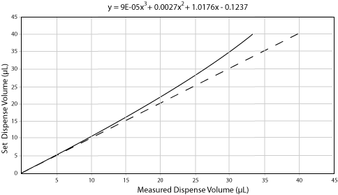 |
The dashed line is a reference line, where the set dispense volume equals the measured dispense volume. The equation is the polynomial for the line, calculated by the spreadsheet program.
6 Enter the curve information into the equation editor of the Liquid Library Editor.
If you repeat the experiment, you will find that the curve is much closer to a straight line. This is because the equation you entered adjusts the action of the servo motor that determines aspirate and dispense volumes, thereby calibrating the dispense.
Using the equation editor
You use the equation editor in the Liquid Library Editor to enter the calibration curve data and correct for pipetting inaccuracy.
To enter a polynomial into the equation editor:
1 Open the Liquid Library Editor.
2 Click the Equation tab to display the equation editor.
3 In the Highest order of polynomial text box, enter the value for the highest order of the polynomial.
This is the largest exponent in the equation and tells you how many terms are in the equation. For example, if the highest order of the polynomial is 3, the equation will have the general form: y = a + bx +cx2 + dx3, where ‘x’ is the volume specified by any pipettor task that uses this liquid class. With an exponent of three, four rows are added to the equation editor table.
4 In the Coefficient/Term table, enter the coefficient and exponent for each of the terms in the equation, starting with the zero order term.
To enter a value, single-click the Coefficient table row twice. Note that the exponents are already entered for you and cannot be edited.
The following example is for the curve displayed in the previous graph.
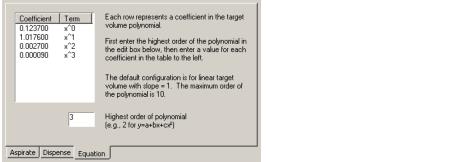 |
5 Click Save changes.
6 VWorks Plus only. If an audit trail is being logged, the Audit Comment dialog box opens. Select or type the audit comment, and then click OK.
Related information
For information about... | See... |
|---|---|
Liquid classes | |
Opening the Liquid Library Editor | |
Creating a liquid class | |
Audit trails and records of interest |